Introduction

The process of image reconstruction is widely used within the medical fields for reconstructing data from a CT scan to show what the inside of a person looks like. This ability to see inside a person allows for doctors to identify problems within the body and treat them appropriately. Another field image re construction is also used in is nondestructive imaging of parts such as on airplanes. This type of imaging allows for checking on the internals of certain structural areas of the plane that would otherwise be expensive as well as damage structural integrity if done. Within this report the basic algorithm for filtered back projecting and comparing this to non-filtered back projections. This type of filter allows for a clearer image after back projecting, and it is the reason why it is filtered. To compare filtered and non-filtered reconstructions a standard reference for computed tomography will be used, the shepp-logan phantom [10].

Applications

The main application of image reconstruction is when an internal view of an object or person is needed but it is either too costly or dangerous to do so. This type of nondestructive and noninvasive view of is useful in several fields. One of the main fields for this is medical imaging. The main use for this type of imaging, is in C.T scanners and MRI machines [11]. These machines allow for noninvasive views in to the body rather than the more invasive biopsy[11]. Another field where tomography is used is within ocean observation, measuring temperatures and currents. This form of tomography use acoustic waves instead of the higher power x-rays as used in medicine [12]. This form of tomography uses the changing speed of sound within the ocean to not only determine ocean temperatures but also depth.

Background

Image reconstruct works because of the “Fourier projection theorem” or Projection-slice theorem” [13]. This theorem states that the integral of a shape projection along some axis is a slice of the 2d Fourier transform of that shape projected along the same axis. A graphical view of this theorem can be seen in Figure 1. This method is called back projection. Plotting all these back projected angles creates a sinogram and example of which can be seen in Figure 2. This figure shows sinogram of a basic test image that can be found in Appendix B: basic image This theorem also states that an infinite number of projects are taken at different angles and the image can be perfectly reconstructed.

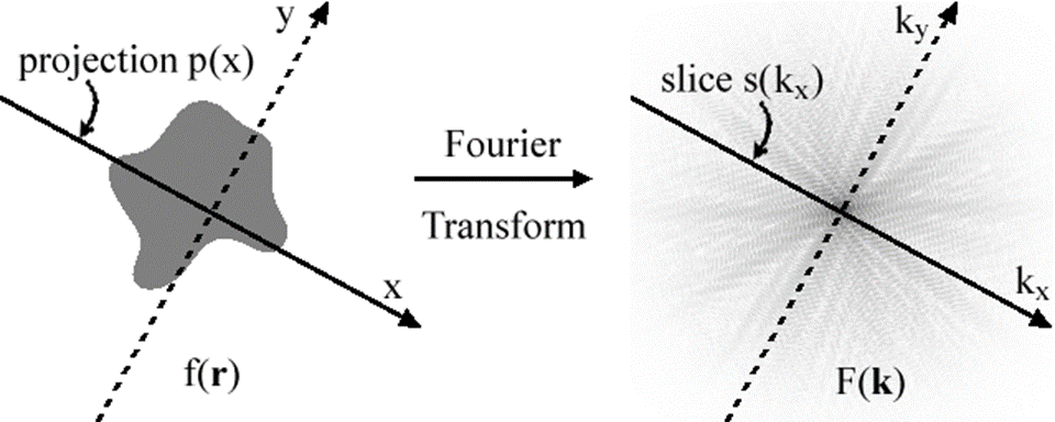Figure 1: example of Fourier projection theorem source: Public Domain, https://commons.wikimedia.org/w/index.php?curid=646788

However, as an infinite number of projections a very large number of angles must be computed to reconstruct the image. Another problem occurs with this projection, as the rotation happens around the origin in Fourier space points near the center in Fourier space have more samples where points further away from the center tend to be more sparsely populated. This is due to the polar sampling in Fourier space. Therefor interpolating between these values is needed to create a clearer image. This is done through a filtering step that uses a ramp filter in the Fourier domain to interpolate between these values.

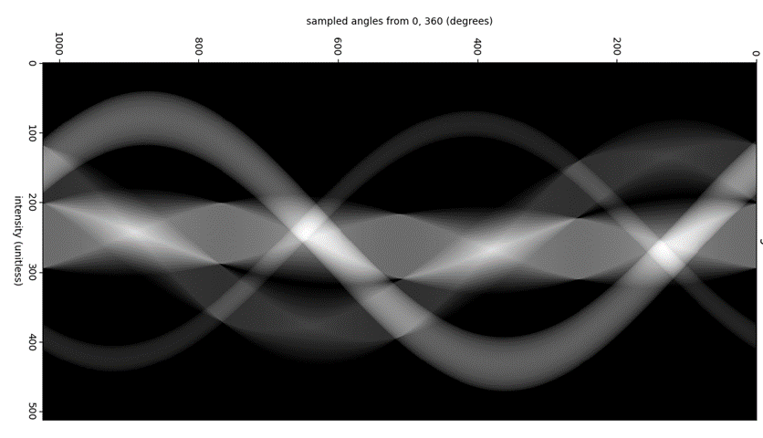Figure 2: sinogram of basic image

As can be seen in this Figure 2: sinogram of basic image the sinogram is mirror at the 180° mark, however it is mirrored both horizontally and vertically. using this knowledge this means that when taking the back projections of an object, only must take the back projections of the object from 0 to 180 degrees to have enough data to reconstruct the object. To take these back projected and reconstructed the image from them a method must be used called forward projection. This technique takes the slice and angle and project the values at that angle across the image plane, as can be seen in Figure 3. 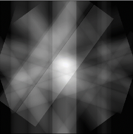Figure 3: forward projection of basic image, with 6 projections

Back projection

As previously discussed with in the Background, to reconstruct and image firstly the image must be back projected to create a sinogram. Although this method will lose value due to polar sampling within the Fourier slice theorem. Using the reference image that was outlined within the Introduction, the sinogram of this image can be seen in Figure 4. The reconstruction from this sinogram can be seen in Figure 5. 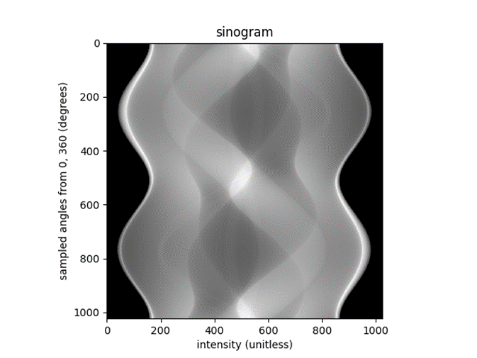Figure 4: sinogram of shepp-logan phantom 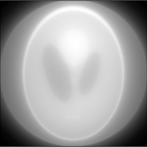Figure 5: reconstruction of shepp-logan phantom This reconstruction is very blur and hard to make out the original image. The reconstruction also has a circle around it most likely from the forward projection stage where the image was rotated and stacked. However, the original shepp-logan phantom can still be made out although some of the smaller details were lost.

Filtered back projection.

The 2d Fourier transform of an image is defined in equation 30:

$$f\left(x,y\right)=\int_{-\infty}^{\infty}\int_{-\infty}^{\infty}F\left(u,v\right){e}^{{j}\mathbf{2\pi}\left({ux}+{vy}\right)}{dudv}\ \ \ \ (1)$$

This equation can then be rewritten using the projection theorem as seen in equation 1:

$${f}\left({x},{y}\right)=\int_{0}^{2\pi}\int_{0}^{\infty}F\left(\delta cos\left(\theta\right),\delta s i n\left(\theta\right)\right){e}^{{j}\mathbf{2\pi}\left(xcos\left(\theta\right)+sin\left(\theta\right){y}\right)}\delta{d}\delta{d}\theta\ \ (2)$$

Simplifying equation 2 further gives equation 3, where p\left(\theta,\delta\right) is the projections of the image defined in equation 1 as f\left(x,y\right). And \left|\delta\right| is the defining the filtering that must be applied to each of the image projections.

$${f}\left({x},{y}\right)=\int_{0}^{2\pi}\int_{0}^{\infty}p\left(\theta,\delta\right){\left|\delta\right|{e}}^{{j}\mathbf{2\pi}\delta r}{d}\delta{d}\theta\ \ \ (3)$$

Using this filter shape that was defined in equation 3, this filter is a ramp filter centering around zero. However, this is a first order filter, and a higher order filter can be used. Although these higher order filters tend to take longer to compute as well as have diminishing returns. This filter is convolved with each of the angle slices. This filter acts as an edge detection filter and increases the amplitude of the signal near the edges of the object. The output of this filter as applied to the first slice can be seen in Figure 6: pre and post filtered slice of the first slice in the sinogram. 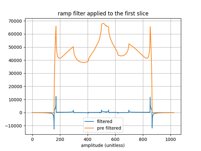Figure 6: pre and post filtered slice of the first slice in the sinogram Applying this filter to the sinogram as seen in Figure 4: sinogram of shepp-logan phantom, creates the sinogram in Figure 7 and reconstructing of this sinogram can be seen in Figure 34. 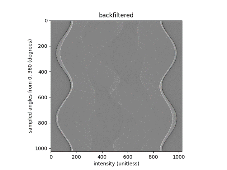Figure 7: sinogram after filtering with ramp filter Figure 8: reconstruction from the sinogram in figure 8 The reconstructed image is sharper with more of the finer details showing through. Although within the image there still is some noise as well as a lack of contrast. The reconstruction also has the same circle around it as the non-filtered reconstruction.

Analysis

Comparing the reconstructions of the images as seen in Figure 5 and Figure 8, the filtered back projection creates a clearer image than the non-filter one. The reasoning for this almost bloom effect on the non-filtered image is the polar sampling in the Fourier slice theorem. This polar sampling causes the bloom effect as there are more samples near the center in Fourier space. These samples near the center correspond to low frequencies, so during the back filtering more lower frequencies samples are captured. This difference in the number of low frequencies captured compared to high frequencies causes most of the details in the image to be lost. These details get lost as these details tend to reside mostly within the higher frequencies in Fourier space. The filter image also shows a noise within the image. This is because the filter that was used is a ramp filter. This type of filter disproportionally amplifies the higher frequency in Fourier space. Although in this case where the higher frequency were the ones that were sample less, the effect is less noticeable. However, this noise could be reduced by using a higher order filter rather than this basic ramp filter. There are also circles that appear around both filtered and non-filtered reconstruction. These circles are more than likely to come from the forward projection stage when the image matrix is rotated. This would occur as during this stage the forward projected image is resampled as well as receiving some interpolation.

Conclusion

In conclusion not filtering the sinogram will lead to a blurry reconstruction with almost a bloom effect to it. although this effect was determined to be caused by the polar sampling of the Fourier slice theorem. Filtering the sinogram creates a sharper reconstruction with a small amount of noise. This noise was found to be from the ramp filter that as used to interpolate the high frequency values what was lost during the polar sampling. However, this noise could be reduced by using a higher order filter. There was also a lighter circle within the reconstruction, and this was determined to be from the interpolation caused by the rotation of the image matrix.

References

[1] H. M. Gach, C. Tanase, and F. Boada, ‘2D & 3D Shepp-Logan Phantom Standards for MRI’, in 2008 19th International Conference on Systems Engineering, IEEE, 2008, pp. 521–526. doi: 10.1109/ICSEng.2008.15. [2] T. Salditt, Biomedical imaging: principles of radiography, tomography and medical physics, 1;1st; Berlin;Boston; De Gruyter, 2017. doi: 10.1515/9783110426694. [3] O. A. Godin, N. A. Zabotin, and V. V. Goncharov, ‘Ocean tomography with acoustic daylight’, Geophysical research letters, vol. 37, no. 13, p. n/a-n/a, 2010, doi: 10.1029/2010GL043623. [4]R. N. Bracewell, ‘Numerical Transforms’, Science (American Association for the Advancement of Science), vol. 248, no. 4956, pp. 697–704, 1990, doi: 10.1126/science.248.4956.697.